T8 : International Journal 1

Judul : Penerapan Aplikasi Pencarian Data Persediaan Obat Berbasis Website Menggunakan Metode K-Means

Constrained K-means Clustering with Background Knowledge 

Abstract 

Clustering is traditionally viewed as an unsupervised method for data analysis. However, in some cases information about the problem domain is available in addition to the data instances themselves. In this paper, we demonstrate how the popular k-means clustering algorithm can be profitably modified to make use of this information. In experiments with artificial constraints on six data sets, we observe improvements in clustering accuracy. We also apply this method to the real-world problem of automatically detecting road lanes from GPS data and observe dramatic increases in performance.

1. Introduction 

Clustering algorithms are generally used in an unsupervised fashion. They are presented with a set of data instances that must be grouped according to some notion of similarity. The algorithm has access only to the set of features describing each object; it is not given any information (e.g., labels) as to where each of the instances should be placed within the partition. 

However, in real application domains, it is often the case that the experimenter possesses some background knowledge (about the domain or the data set) that could be useful in clustering the data. Traditional clustering algorithms have no way to take advantage of this information even when it does exist. 

We are therefore interested in ways to integrate background information into clustering algorithms. We have previously had success with a modified version of COBWEB (Fisher, 1987) that uses background information about pairs of instances to constrain their cluster placement (Wagstaff & Cardie, 2000). K-means is another popular clustering algorithm that has been used in a variety of application domains, such as image segmentation (Marroquin & Girosi, 1993) and information retrieval (Bellot & El-Beze, 1999). Due to its widespread use, we believe that developing a modified version that can make use of background knowledge can be of significant use to the clustering community. 

The major contributions of the current work are twofold. First, we have developed a k-means variant that can incorporate background knowledge in the form of instance-level constraints, thus demonstrating that this approach is not limited to a single clustering algorithm. In particular, we present our modifications to the k-means algorithm and demonstrate its performance on six data sets. 

Second, while our previous work with COBWEB was restricted to testing with random constraints, we demonstrate the power of this method applied to a significant real-world problem (see Section 6). 

In the next section, we provide some background on the k-means algorithm. Section 3 examines in detail the constraints we propose using and presents our modified k-means algorithm. Next, we describe our evaluation methods in Section 4. We present experimental results in Sections 5 and 6. Finally, Section 7 compares our work to related research and Section 8 summarizes our contributions.

2. K-means Clustering 

K-means clustering (MacQueen, 1967) is a method commonly used to automatically partition a data set into k groups. It proceeds by selecting k initial cluster centers and then iteratively refining them as follows:

1. Each instance di is assigned to its closest cluster center. 

2. Each cluster center Cj is updated to be the mean of its constituent instances. 

The algorithm converges when there is no further change in assignment of instances to clusters. 

In this work, we initialize the clusters using instances chosen at random from the data set. The data sets we used are composed solely of either numeric features or symbolic features. For numeric features, we use a Euclidean distance metric; for symbolic features, we compute the Hamming distance. 

The final issue is how to choose k. For data sets where the optimal value of k is already known (i.e., all of the UCI data sets), we make use of it; for the realworld problem of finding lanes in GPS data, we use a wrapper search to locate the best value of k. More details can be found in Section 6.

3. Constrained K-means Clustering 

We now proceed to a discussion of our modifications to the k-means algorithm. In this work, we focus on background knowledge that can be expressed as a set of instance-level constraints on the clustering process. After a discussion of the kind of constraints we are using, we describe the constrained k-means clustering algorithm. 

3.1 The Constraints 

In the context of partitioning algorithms, instancelevel constraints are a useful way to express a priori knowledge about which instances should or should not be grouped together. Consequently, we consider two types of pairwise constraints: 

      • Must-link constraints specify that two instances have to be in the same cluster. 

      • Cannot-link constraints specify that two instances must not be placed in the same cluster. 

The must-link constraints define a transitive binary relation over the instances. Consequently, when making use of a set of constraints (of both kinds), we take a transitive closure over the constraints.1 The full set of derived constraints is then presented to the clustering algorithm. In general, constraints may be derived from partially labeled data (cf. Section 5) or from background knowledge about the domain or data set (cf. Section 6).

3.2 The Constrained Algorithm 

Table 1 contains the modified k-means algorithm (COP-KMEANS) with our changes in bold. The algorithm takes in a data set (D), a set of must-link constraints (Con=), and a set of cannot-link constraints (Con6=). It returns a partition of the instances in D that satisfies all specified constraints. 

The major modification is that, when updating cluster assignments, we ensure that none of the specified constraints are violated. We attempt to assign each point di to its closest cluster Cj . This will succeed unless a constraint would be violated. If there is another point d= that must be assigned to the same cluster as d, but that is already in some other cluster, or there is another point d6= that cannot be grouped with d but is already in C, then d cannot be placed in C. We continue down the sorted list of clusters until we find one that can legally host d. Constraints are never broken; if a legal cluster cannot be found for d, the empty partition ({}) is returned. An interactive demo of this algorithm can be found at http://www.cs.cornell.edu/home/wkiri/cop-kmeans/.

4. Evaluation Method 

The data sets used for the evaluation include a “correct answer” or label for each data instance. We use the labels in a post-processing step for evaluating performance. 

To calculate agreement between our results and the correct labels, we make use of the Rand index (Rand, 1971). This allows for a measure of agreement between two partitions, P1 and P2, of the same data set D. Each partition is viewed as a collection of n∗ (n−1)/2 pairwise decisions, where n is the size of D. For each pair of points di and dj in D, Pi either assigns them to the same cluster or to different clusters. Let a be the number of decisions where di is in the same cluster as dj in P1 and in P2. Let b be the number of decisions where the two instances are placed in different clusters in both partitions. Total agreement can then be calculated using

We used this measure to calculate accuracy for all of our experiments. We were also interested in testing our hypothesis that constraint information can boost performance even on unconstrained instances. Consequently, we present two sets of numbers: the overall accuracy for the entire data set, and accuracy on a held-out test set (a subset of the data set composed of instances that are not directly or transitively affected by the constraints). This is achieved via 10-fold crossvalidation; we generate constraints on nine folds and evaluate performance on the tenth. This enables a true measurement of improvements in learning, since any improvements on the held-out test set indicate that the algorithm was able to generalize the constraint information to the unconstrained instances as well.

5. Experimental Results Using Artificial Constraints 

In this section, we report on experiments using six well-known data sets in conjunction with artificiallygenerated constraints. Each graph demonstrates the change in accuracy as more constraints are made available to the algorithm. The true value of k is known for these data sets, and we provided it as input to our algorithm. 

The constraints were generated as follows: for each constraint, we randomly picked two instances from the data set and checked their labels (which are available for evaluation purposes but not visible to the clustering algorithm). If they had the same label, we generated a must-link constraint. Otherwise, we generated a cannot-link constraint. We conducted 100 trials on each data set (where a trial is one 10-fold cross validation run) and averaged the results. 

In our previous work with COP-COBWEB, a constrained partitioning variant of COBWEB, we made use of three UCI data sets (soybean, mushroom, and tic-tac-toe) and one “real-world” data set that involved part of speech data (Wagstaff & Cardie, 2000). In this work, we replicated our COP-COBWEB experiments for the purpose of comparison with COP-KMEANS. COBWEB is an incremental algorithm, while k-means is a batch algorithm. Despite their significant algorithmic differences, we found that both algorithms improved almost identically when supplied with the same amount of background information.

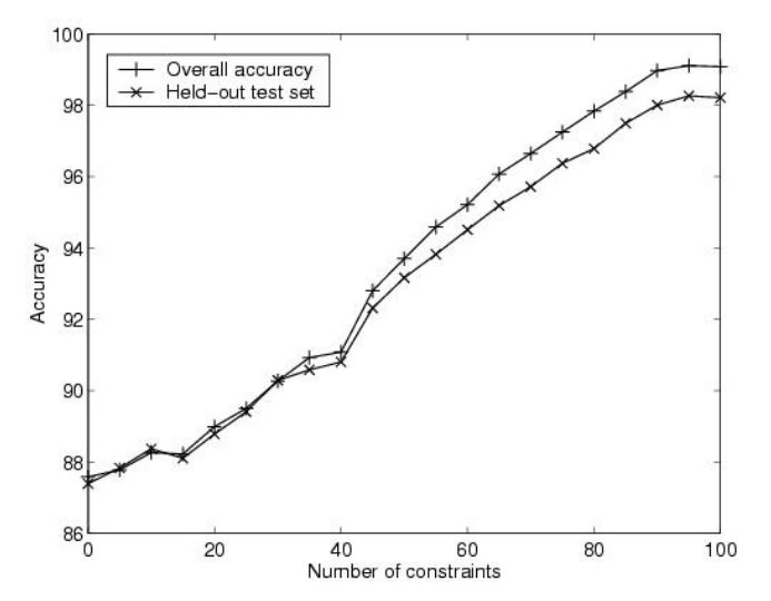
Figure 1. COP-KMEANS results on soybean 

The first data set of interest is soybean, which has 47 instances and 35 attributes. Four classes are represented in the data. Without any constraints, the k-means algorithm achieves an accuracy of 87% (see Figure 1). Overall accuracy steadily increases with the incorporation of constraints, reaching 99% after 100 random constraints. 

We applied the Rand index to the set of constraints vs. the true partition. Because the Rand index views a partition as a set of pairwise decisions, this allowed us to calculate how many of those decisions were ’known’ by the set of constraints.2 For this data set, 100 random constraints achieve an average accuracy of 48%. We can therefore see that combining the power of clustering with background information achieves better performance than either in isolation

Held-out accuracy also improves, achieving 98% with 100 constraints. This represents a held-out improvement of 11% over the baseline (no constraints). Similarly, COP-COBWEB starts at 85% accuracy with no constraints, reaching a held-out accuracy of 96% with 100 random constraints.3

Figure 2. COP-KMEANS results on mushroom 

We next turn to the mushroom data set, with 50 instances and 21 attributes.4 It contains two classes. In the absence of constraints, the k-means algorithm achieves an accuracy of 69% (Figure 2). After incorporating 100 random constraints, overall accuracy improves to 96%. In this case, 100 random constraints achieve 73% accuracy before any clustering occurs. Held-out accuracy climbs to 82%, yielding an improvement of 13% over the baseline. COP-COBWEB starts at 67% accuracy with no constraints, with held-out accuracy reaching 83% with 100 constraints. 

The third data set under consideration is the part-ofspeech data set (Cardie, 1993). A subset of the full data set, it contains 50 instances, each described by 28 attributes. There are three classes in this data set. Without constraints, the k-means algorithm achieves an accuracy of 58% (We have omitted the graph for this data set, as COP-KMEANS and COP-COBWEB have very similar performance, just as shown in the previous two figures.). After incorporating 100 random constraints, overall accuracy improves to 87%. Here, 100 random constraints attain 56% accuracy. Held-out accuracy climbs to 70%, yielding an improvement of 12% over the baseline. Likewise, COP COBWEB starts at 56% accuracy with no constraints, reaching a held-out accuracy of 72% with 100 constraints.

Figure 3. COP-KMEANS results on tic-tac-toe 

Finally, we focus on the tic-tac-toe data set.5 There are 100 instances in this data set, each described by 9 attributes. There are two classes in this data set. Without constraints, the k-means algorithm achieves an accuracy of 51% (Figure 3). After incorporating 500 random constraints, overall accuracy is 92%. This set of constraints achieves 80% accuracy in isolation. Held-out accuracy reaches 56%, achieving a 5% increase in accuracy. 

COP-COBWEB behaves somewhat worse on this data set, with held-out performance staying roughly at the 49% mark. We believe that this data set is particularly challenging because the classification of a board as a win or a loss for the X player requires extracting relational information between the attributes — information not contained in our instance-level constraints. 

In contrast to the COP-COBWEB experiments, which made use of data sets with symbolic (categorical) attributes, we also experimented with using COPKMEANS on two UCI data sets with numeric (continuous) attributes. On the iris data set (150 instances, four attributes, three classes), incorporating 400 random constraints yielded a 7% increase in held-out accuracy. Overall accuracy climbed from 84% to 98%, and the set of constraints achieved 66% accuracy. Behavior on the wine data set (178 instances, 13 attributes, three classes) was similar to that of the tictac-toe data set, with only marginal held-out improvement (although overall accuracy, as usual, increased dramatically, from 71% to 94%). The constraint set achieved 68% in isolation. 

What we can conclude from this section is that even randomly-generated constraints can improve clustering accuracy. As one might expect, the improvement obtained depends on the data set under consideration. If the constraints are generalizable to the full data set, improvements can be observed even on unconstrained instances.

6. Experimental Results on GPS Lane Finding 

In all of the above experiments, the constraints we experimented with were randomly generated from the true data labels. To demonstrate the utility of constrained clustering with real domain knowledge, we applied COP-KMEANS to the problem of lane finding in GPS data. In this section, we report on the results of these experiments. More details can be found in Schroedl et al. (2001), which focuses specifically on the problem of map refinement and lane finding. 

As we will show, the unconstrained k-means algorithm performs abysmally compared to COP-KMEANS, which has access to additional domain knowledge about the problem. Section 6.2 describes how we transformed this domain knowledge into a useful set of instance-level constraints. 

6.1 Lane Finding Explained 

Digital road maps currently exist that enable several applications, such as generating personalized driving directions. However, these maps contain only coarse information about the location of a road. By refining maps down to the lane level, we enable a host of more sophisticated applications such as alerting a driver who drifts from the current lane. 

Our approach to this problem is based on the observation that drivers tend to drive within lane boundaries. Over time, lanes should correspond to “densely traveled” regions (in contrast to the lane boundaries, which should be “sparsely traveled”). Consequently, we hypothesized that it would be possible to collect data about the location of cars as they drive along a given road and then cluster that data to automatically determine where the individual lanes are located. 

We collected data approximately once per second from several drivers using GPS receivers affixed to the top of the vehicle being driven. Each data point is represented by two features: its distance along the road segment and its perpendicular offset from the road centerline.6 For evaluation purposes, we asked the drivers to indicate which lane they occupied and any lane changes. This allowed us to label each data point with its correct lane.

6.2 Background Knowledge as Constraints 

For the problem of automatic lane detection, we focused on two domain-specific heuristics for generating constraints: trace contiguity and maximum separation. These represent knowledge about the domain that can be encoded as instance-level constraints. 

Trace contiguity means that, in the absence of lane changes, all of the points generated from the same vehicle in a single pass over a road segment should end up in the same lane. 

Maximum separation refers to a limit on how far apart two points can be (perpendicular to the centerline) while still being in the same lane. If two points are separated by at least four meters, then we generate a constraint that will prevent those two points from being placed in the same cluster. 

To better analyze performance in this domain, we modified the cluster center representation. The usual way to compute the center of a cluster is to average all of its constituent points. There are two significant drawbacks of this representation. First, the center of a lane is a point halfway along its extent, which commonly means that points inside the lane but at the far ends of the road appear to be extremely far from the cluster center. Second, applications that make use of the clustering results need more than a single point to define a lane. 

Consequently, we instead represented each lane cluster with a line segment parallel to the centerline. This more accurately models what we conceptualize as “the center of the lane”, provides a better basis for measuring the distance from a point to its lane cluster center, and provides useful output for other applications. Both the basic k-means algorithm and COP-KMEANS make use of this lane representation (for this problem). 

6.3 Experiment 1: Comparison with K-means 

Table 2 presents accuracy results7 for both algorithms over 20 road segments. The number of data points for each road segment is also indicated. These data sets

are much larger than the UCI data sets, providing a chance to test the algorithms’ scaling abilities. 

In these experiments, the algorithms were required to select the best value for the number of clusters, k. To this end, we used a second measure that trades off cluster cohesiveness against simplicity (i.e., number of clusters).8 Note that this measure differs from the objective function used by k-means and COP-KMEANS while clustering. In the language of Jain and Dubes (1988), the former is a relative criterion, while the latter is an internal criterion. 

In the lane finding domain, the problem of selecting k is particularly challenging due to the large amount of noise in the GPS data. Each algorithm performed 30 randomly-initialized trials with each value of k (from 1 to 5). COP-KMEANS selected the correct value for k for all but one road segment, but k-means never chose the correct value for k (even though it was using the same method for selecting k). As shown in Table 2, COP-KMEANS consistently outperformed the unconstrained k-means algorithm, attaining 100% accuracy for all but three data sets 8More precisely, it calculates the average squared distance from each point to its assigned cluster center and penalizes for the complexity of the solution: Σi dist(di,di.cluster) 2 n ∗k 2 . The goal is to minimize this value and averaging 98.6% overall. The unconstrained version performed much worse, averaging 58.0% accuracy. The clusters the latter algorithm produces often span multiple lanes and never cover the entire road segment lengthwise. Lane clusters have a very specific shape: they are greatly elongated and usually oriented horizontally (with respect to the road centerline). Yet even when the cluster center is a line rather than a point, k-means seeks compact, usually spherical clusters. Consequently, it does a very poor job of locating the true lanes in the data. 

For example, Figure 4 shows the output of the regular k-means algorithm for data set 6.9 The horizontal axis is the distance along the road (in meters) and the vertical axis is the centerline offset. There are four true lanes. The points for each of the four clusters found by k-means are represented by different symbols. Clearly, these lanes do not correspond to the true lanes.

Figure 4. K-means output for data set 6, k=4 

The final column in Table 2 is a measure of how much is known after generating the constraints and before doing any clustering. It shows that an average accuracy of 50.4% can be achieved using the background information alone. What this demonstrates is that neither general similarity information (k-means clustering) nor domain-specific information (constraints) alone perform very well, but that combining the two sources of information effectively (COP-KMEANS) can produce excellent results. 

An analysis of the errors made by COP-KMEANS on the lane-finding data sets showed that each mistake arose for a different reason. For data set 12, the algorithm incorrectly included part of a trace from lane 4 in lane 3. This appears to have been caused by noise in the GPS points in question: they are significantly closer to lane 3 than lane 4. On data set 16, COPKMEANS chose the wrong value for k (it decided on three lanes rather than four). This road segment contains very few traces, which possibly contributed to the difficulty. Since COP-KMEANS made so few errors on this data set, it is not possible to provide a more general characterization of their causes. 

It might be argued that k-means is simply a poor choice of algorithm for this problem. However, the marked improvements we observed with COPKMEANS suggest another advantage of this method: algorithm choice may be of less importance when you have access to constraints based on domain knowledge. For this task, even a poorly-performing algorithm can boost its performance to extremely high levels. In essence, it appears that domain knowledge can make performance less sensitive to which algorithm is chosen. 

6.4 Experiment 2: Comparison with agglom 

Rogers et al. (1999) previously experimented with a clustering approach that viewed lane finding as a onedimensional problem. Their algorithm (agglom) only made use of the centerline offset of each point. They used a hierarchical agglomerative clustering algorithm that terminated when the two closest clusters were more than a given distance apart (which represented the maximum width of a lane). 

This approach is quite effective when there are no lane merges or splits across a segment, i.e., each lane continues horizontally from left to right with no interruptions. For the data sets listed in Table 2, their algorithm obtains an average accuracy of 99.4%.10 

However, all of these data sets were taken from a freeway, where the number of lanes is constant over the entirety of each road segment. In cases where there are lane merges or splits, the one-dimensional approach is inadequate because it cannot represent the extent of a lane along the road segment. We are currently in the process of obtaining data for a larger variety of roads, including segments with lane merges and splits, which we expect will illustrate this difference more clearly. 

7. Related Work 

A lot of work on certain varieties of constrained clustering has been done in the statistical literature (Gordon, 1973; Ferligoj & Batagelj, 1983; Lefkovitch, 1980). In general, this work focuses exclusively on agglomerative clustering algorithms and contiguity constraints (similar to the above trace contiguity constraint). In particular, no accommodation is provided for constraints that dictate the separation of two items. In addition, the contiguity relation is assumed to cover all data items. This contrasts with our approach, which can easily handle partial constraint relations that only cover a subset of the instances. 

In the machine learning literature, Thompson and Langley (1991) performed experiments with providing an initial “priming” concept hierarchy to several incremental unsupervised clustering systems. The algorithms were then free to modify the hierarchy as appropriate. In contrast to these soft constraints, our approach focuses on hard, instance-level constraints. 

Additionally, Talavera and B´ejar incorporated domain knowledge into an agglomerative algorithm, ISAAC (Talavera & Bejar, 1999). It is difficult to classify ISAAC’s constraints as uniformly hard or soft. The final output is a partition (from some level of the hierarchy), but the algorithm decides at which level of the hierarchy each constraint will be satisfied. Consequently, a given constraint may or may not be satisfied by the output. 

It is possible for the k-means algorithm to evolve empty clusters in the course of its iterations. This is undesirable, since it can produce a result with fewer than k clusters. Bradley et al. (2000) developed a method to ensure that this would never happen by imposing a minimum size on each cluster. Effectively, these act as cluster-level constraints. Like our instance-level constraints, they can be used to incorporate domain knowledge about the problem. For example, we know that road lanes must be separated by some minimum distance. However, we have not yet incorporated this type of constraint as an input to the clustering algorithm; rather, we simply discard solutions that contain lanes that are deemed too close together. We are interested in exploring these clusterlevel constraints and integrating them more closely with the clustering algorithm itself.

8. Conclusions and Future Directions 

We have developed a general method for incorporating background knowledge in the form of instancelevel constraints into the k-means clustering algorithm. In experiments with random constraints on six data sets, we have shown significant improvements in accuracy. Interestingly, the results obtained with COPKMEANS are very similar to those obtained with COP-COBWEB. In addition, we have demonstrated how background information can be utilized in a real domain, GPS lane finding, and reported on impressive gains in accuracy. 

We see several avenues for improvements and future work. The use of constraints while clustering means that, unlike the regular k-means algorithm, the assignment of instances to clusters can be order-sensitive. If a poor decision is made early on, the algorithm may later encounter an instance di that has no possible valid cluster (e.g., it has a cannot-link constraint to at least one item in each of the k clusters). This occasionally occurred in our experiments (for some of the random data orderings). Ideally, the algorithm would be able to backtrack, rearranging some of the instances so that di could then be validly assigned to a cluster. 

Additionally, we are interested in extending the constrained clustering approach to include hierarchical algorithms. COP-KMEANS and COP-COBWEB both generate a partition of the data and therefore are wellsituated to take advantage of hard, instance-level constraints. A different constraint formulation will be required for hierarchical algorithms. 

Finally, we would like to explore an alternative to the hard constraints presented here. Often domain knowledge is heuristic rather than exact, and it is possible that it would be better expressed by a “soft” constraint

Acknowledgements 

We thank Pat Langley for his assistance and suggestions and for access to the GPS data sets. We would especially like to thank Westley Weimer for advice and suggestions on the work as it progressed. We also thank Marie desJardins for her insightful comments.

sumber: https://web.cse.msu.edu/~cse802/notes/ConstrainedKmeans.pdf